積分

　プログラミングの基本的で重要なアプリケーションの1つは、積分と導関数です。微積分の講義で学んだように、線形、二次、多項式、三角関数などの関数は解析的に積分を行うことができますが、その一方で他の多くの関数については解析的に積分をすることできません。そのような時に利用するのが数値積分です。数値積分を利用すれば、ほとんどの場合に積分を実行することができます。

一般的な積分について

　関数 \(f(x)\) があり、\(x\) に関する \(x\) = a から \(x\) = b までの積分を計算したいとします。これを \(I(a, b)\) とします。

\[I(a,b) = \int_a^b f(x)dx\]

　これは、a から b までの \(f(x)\) の曲線の下の面積を計算することと同じです。

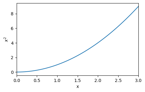
　簡単な例から始めます。0 < \(x\) < 3 上の \(x^2\) で積分を試みます。

%matplotlib inline

import matplotlib.pyplot as plt
import numpy as np

x = np.linspace(0,3,100)
y = x*x

plt.figure(figsize=(5,3))
plt.plot(x,y)
plt.xlabel('x')
plt.ylabel('$x^2$')
plt.xlim([0,3])
plt.show()

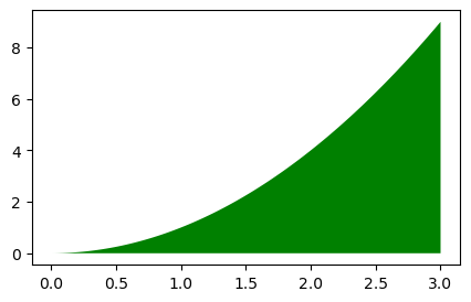
　数学的には、積分は曲線の下の面積を意味します

y0 = np.zeros(100)

plt.figure(figsize=(5,3))
plt.fill_between(x, y0, y, where=y>=y0, facecolor='green')
plt.show()

　このような面積をコンピュータを使って計算する方法を考えます。以下の２点について考えてみましょう。

• 面積を近似的に見積もる方法

• より正確に計算するには？

長方形近似

　面積を求める最も簡単な方法は次のとおりです。

1. 領域を多数の長方形に分割

2. それぞれの長方形の面積を計算

3. それらを足し合わせる

　このような近似法を長方形近似といいます。長方形近似で面積を計算する関数Rectangleを下記のように定義します。

import numpy as np
import matplotlib.pyplot as plt

def Rectangle(start, end, parts):
    """
    Rectrangle sum rule

    """

    #define the function
    f = lambda x: x * x

    #define the X,Y points
    deltax = (end - start) / parts
    resultsx = np.linspace(start, end, parts)
    resultsy = f(resultsx)

    # To calculate the area
    area = np.empty([parts], float)
    for i in range(parts):
            area[i] = resultsy[i] * deltax
    return sum(area)

　startとendは積分の範囲、partsは分割数を指定します。

def Rectangle_plot(start, end, parts):
    #define the function
    f = lambda x: x * x

    #define the X,Y points
    deltax = (end - start) / parts
    resultsx = np.linspace(start, end, parts)
    resultsy = f(resultsx)

    x = np.linspace(start,end,100)
    y = x*x
    plt.plot(x, y, 'r')
    plt.xlim([start,end])
    plt.bar(resultsx+deltax/2, resultsy, deltax, edgecolor ='black')
    #plt.bar(resultsx, resultsy, deltax, edgecolor ='black')
    plt.show()
    #print("The Sum of the area is: ", sum(area))

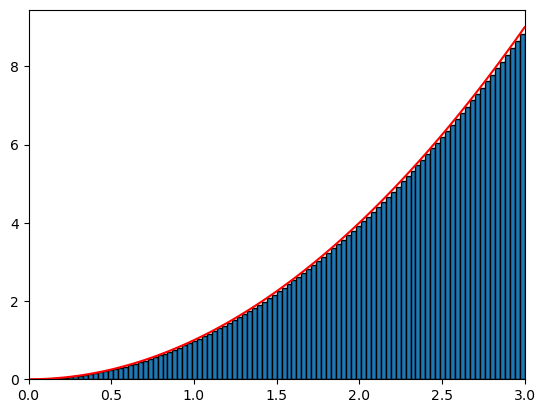
　0 ~ 3までの間を100個に分割して面積を求めるには以下のようにします。

Rectangle(0,3,100)

9.045454545454543

Rectangle_plot(0,3,100)

0 ~ 3までの間を20個に分割して面積を求めます。

Rectangle(0,3,20)

9.236842105263156

Rectangle_plot(0,3,20)

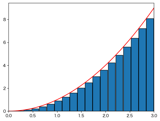
　どちらが正確な値をだしているでしょうか。

Rectangle(0,3,100)
Rectangle_plot(0,3,100)

台形公式

　長方形近似は比較的簡単に計算することができますが、かなり大雑把な計算です。

　より良い方法は、長方形ではなく台形を使用することです。この方法は単純ですが、多くの場合十分な結果が得られます。

　台形近似で面積を計算する関数Trapezoidを下記のように定義します。

import numpy as np
import matplotlib.pyplot as plt

def Trapezoid(start, end, parts):
    """
    Trapezoid sum rule

    """
    #define the function
    f = lambda x: x * x

    #define the X, Y points
    deltax = (end - start) / parts
    resultsx = np.linspace(start, end, parts+1)
    resultsy = f(resultsx)

    # To calculate the area
    area = np.empty([parts], float)
    for i in range(parts):
            area[i] = (resultsy[i]+resultsy[i+1]) * deltax/2
    return sum(area)

def Trapezoid_plot(start, end, parts):
    #define the function
    f = lambda x: x * x

    #define the X, Y points
    deltax = (end - start) / parts
    resultsx = np.linspace(start, end, parts+1)
    resultsy = f(resultsx)

    x = np.linspace(start,end,100)
    y = f(x)
    plt.plot(x, y, 'r')
    plt.xlim([start,end])

    y2 = np.array([0,0])
    for i in range(parts):
        x0 = resultsx[i:i+2]
        y1 = resultsy[i:i+2]
        plt.fill_between(x0, y1, y2, where=y1>=y2, facecolor='blue')
        linex, liney = [resultsx[i+1], resultsx[i+1]], [0, resultsy[i+1]]
        plt.plot(linex, liney, color='black', linewidth=2.0)

    plt.show()
    #print("The Sum of the area is: ", sum(area))

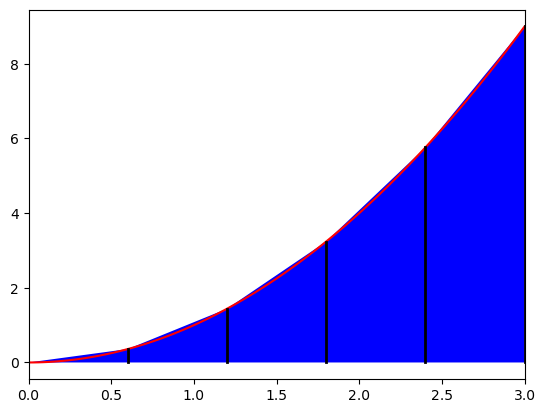
0 ~ 3までの間を５個に分割して面積を求めます。

Trapezoid(0,3,5)

9.045

Trapezoid_plot(0,3,5)

0 ~ 3までの間を１０個に分割して面積を求めます。

Trapezoid(0,3,10)

9.045

Trapezoid_plot(0,3,10)

　台形近似の高い精度を確認することができます。

シンプソンの公式

　台形公式は単純で、これまで見てきたように数行のコードしか必要としません。高い精度が必要とされない計算には適しています。

　より高い精度が必要な場合にはどうしたら良いでしょうか。計算に使用するステップ数 N を増やすことで精度を上げることができます。

　ただし場合によっては、計算が遅くなることがあります。積分を高い精度を維持しながらすばやく答えを得ることができるでしょうか。

　積分する関数を、曲線で近似するとより良い結果が得られることがあります。シンプソンの公式は、二次曲線を使用してこれを行います。二次方程式を完全に指定するには、直線のように 2 点だけでなく、3 点が必要です。

　被積分関数が \(f(x)\) で示され、隣接する点の間隔が \(h\) で、\(x\) = −\(h\)、0、および +\(h\) に 3 つの点があるとします。 これらの点を通る 2 次 \(Ax^2 + Bx + C\) を当てはめると、定義により次のようになります。

\[f(-h) = Ah^2 - Bh + C\]

\[f(0) = C\]

\[f(h) = Ah^2 + Bh + C\]

　これらの方程式を解くと、

\[A = \frac{1}{h^2}[\frac{f(-h)}{2} - f(0) + \frac{f(h)}{2}]\]

\[B=\frac{1}{2h}[f(h)-f(-h)]\]

\[C = f(0)\]

　−\(h\) から +\(h\) までの \(f(x)\) の曲線の下の面積は、二次方程式の下の面積によって近似的に与えられます。

\[\int^h_{-h} (Ax^2 + Bx + C) dx = \frac{2}{3}Ah^3 + 2Ch = \frac{1}{3}h[f(-h)+4f(0)+f(h)]\]

　これがシンプソンの公式です。これにより、関数の隣接する 2 つのスライスの下の領域の近似値が得られます。

　面積の式は、ちょうど台形規則と同様に、\(h\) と等間隔の点での関数の値のみを含みます。したがって、シンプソンの公式を使用する場合に、二次方程式の詳細について心配する必要はありません。数値をこの式に代入するだけで答えを得ることができます。

　シンプソンの公式を適用するには、まず積分領域を分割します。続いてこの公式を使用して連続する分割領域の面積を計算し、すべての領域の面積を加算して全面積を得ます。

　幅 \(h\) のスライスで \(x\) = a から \(x\) = b までを統合する場合、最初の領域の 3 つの点は、\(x = a、a + h、a + 2h\)です。

　2 番目の領域は\(a + 2h、a + 3h、a + 4h\) になります。

　積分全体の近似値は次のように与えられます。

\[\begin{split}\begin{aligned} I(a,b) \approx & \frac{1}{3}h[f(a)+4f(a+h)+f(a+2h)] \\ & + \frac{1}{3}h[f(a+2h)+4f(a+3h)+f(a+4h)] \\ & +...\\ & +...\\ & + \frac{1}{3}h[f(a+(N-2)h)+4f(a+(N-1)h)+f(b)] \end{aligned}\end{split}\]

see more details in: https://en.wikipedia.org/wiki/Simpson%27s_rule

課題１：シンプソンの公式

　以下のコードを、シンプソン公式の関数を定義して完成させてください。

import numpy as np
import matplotlib.pyplot as plt

def Simpson(start, end, parts, plot=1):
    """
    Simpson sum rule

    """
    #define the function
    f = lambda x: x**4 - 2*x + 1

    #define the X, Y points
    deltax = (end - start) / parts
    resultsx = np.linspace(start, end, parts+1)
    resultsy = f(resultsx)

    #-----------------------------------------------------
    #define the Simpson points and calculate the area here
    #-----------------------------------------------------
    area = []

    #By default, we also output the plot.
    if plot==1:
        x = np.linspace(start,end,100)
        y = f(x)
        plt.plot(x, y, 'r')

        #-----------------------------------------------------
        #draw the curves based on Simpson points here
        #-----------------------------------------------------

        plt.xlim([start,end])
        plt.ylim([min(y),max(y)])
        plt.show()

    return sum(area)

課題２：積分計算

　長方形近似、台形近似、シンプソンの公式を使用して、次の積分を計算してください。

\[\int_0^3 (x^2-x+1 dx)\]

\[\int_0^3 (x^4-x+1 dx)\]

\[\int_0^3 \text{exp}(-x^2) dx\]

　シンプソンの公式を使う場合、いくつのサンプリングポイントが必要になるか考えてみましょう？

発展：高次へのさらなる展開

　これまで見てきたように、台形公式は被積分関数 \(f(x)\) を直線で近似することに基づいていますが、シンプソンの公式は二次方程式を使用しています。高次の多項式を使用し、\(f(x)\) を3次や4次などでフィッティングすることにより、高次の (より正確な) 積分公式を作成できます。

台形公式とシンプソンの公式の一般的な形式は次のとおりです。

\[\int_a^b f(x)dx \approx \sum_{k=1}^{N}w_kf(k)\]

ここで、\(x_k\) は被積分関数を計算するサンプル ポイントの位置であり、\(w_k\) は重みのセットです。

• 台形公式では、最初と最後の重みは 1/2 で、他はすべて 1 です。

• シンプソンの公式では、最初と最後のスライスの重みは1/3で、他のスライスの重みは4/3と2/3の間で交互になります。

次数	近似法	係数
0	長方形	1,1,……..1,1
1	直線	1/2,1,1,…..1,1/2
2	二次曲線	1/3, 4/3, 2/3, ..,4/3,1/3
3	三次曲線	……………….

発展：ガウス求積法

　ここまでサンプルポイントは等間隔であると仮定しており、これにより比較的簡単にプログラムを作成することができます。一方で、点の間隔が不均一な積分法を導出することもできます。場合によっては、少数の点数で非常に正確な答えを出すこともできます。これには Gaussian Quadrature と呼ばれるよく知られた方法があります。

Gaussian Quadrature を数学の基礎から紹介する wiki ページ。 https://ja.wikipedia.org/wiki/ガウス求積

from numpy import ones,copy,cos,tan,pi,linspace

def gaussxw(N):

    # Initial approximation to roots of the Legendre polynomial
    a = linspace(3,4*N-1,N)/(4*N+2)
    x = cos(pi*a+1/(8*N*N*tan(a)))

    # Find roots using Newton's method
    epsilon = 1e-15
    delta = 1.0
    while delta>epsilon:
        p0 = ones(N,float)
        p1 = copy(x)
        for k in range(1,N):
            p0,p1 = p1,((2*k+1)*x*p1-k*p0)/(k+1)
        dp = (N+1)*(p0-x*p1)/(1-x*x)
        dx = p1/dp
        x -= dx
        delta = max(abs(dx))

    # Calculate the weights
    w = 2*(N+1)*(N+1)/(N*N*(1-x*x)*dp*dp)

    return x,w


def f(x):
    return x**5 - 2*x + 1

N = 3
a,b = 0.0, 2.0

# Calculate the sample points and weights, then map them
# to the required integration domain
x,w = gaussxw(N)
xp = 0.5*(b-a)*x + 0.5*(b+a)
wp = 0.5*(b-a)*w

# Perform the integration
s = 0.0
for k in range(N):
    s += wp[k]*f(xp[k])
print(s)

8.666666666666684

scipy の組み込み関数

https://docs.scipy.org/doc/scipy/reference/integrate.html#module-scipy.integrate

from scipy import integrate
f = lambda x: x * x
integrate.quad(f, 1, 3)