最小二乗フィッティング
カーブフィッティングは、データ解析よく用いられます。補間と同様に特定のデータポイントに基づいて関数を近似しますが、関数を近似する基準が異なります。
補間は、指定されたデータポイントの値を必ず通ります。
フィッティングは、指定されたデータポイントの値を必ず通るわけではなく、一般的な関数を使用して全体像を記述しようとします。
いろいろなところで目にするように、補完とフィッティングの間には多くの共通の数学があります。
[32]:
import matplotlib.pyplot as plt
import numpy as np

#define the function
f = lambda x: 3*x+2

#define the paramters for the plot
a,b = 0,3
npoints = 10

x = np.linspace(a,b,npoints)
y = f(x) + np.random.rand(npoints) - 0.5

plt.plot(x,y, 'o', label='noisy data')
plt.plot(x,f(x), '-', label='fit1')
plt.plot(x,4*x+1, '--', label='fit2')

plt.xlabel('x')
plt.ylabel('$f(x)$')
plt.xlim([a,b])
plt.legend()
plt.show()
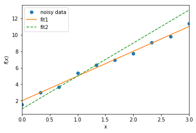
上の図は、y=3x+2という一次関数に対してランダムなノイズを加えて10個の点を生成し、プロットしたものです。
オレンジの線はy=3x+2を示しているので、各点の近くを通る線となっています。
それに対して点線は、y=4x+1という一次関数を示しています。x=1から離れると、各点から離れていくことがわかります。
この結果から、当然ですが、y=3x+2のほうが良いフィッティングであることがわかります。
フィッティングの評価基準
それではどのようなフィッティングがよいフィッティングかを考えてみましょう。以下のような一連の点があるとします。
これらの点を最もよく表す直線 \(f(x) = ax+b\) を描きたいとします。\(a\) と \(b\) には任意の数を選択できます。この\(a\) と \(b\) を選択する際に最も良いの基準はどんなものでしょうか。
フィッティングのエラーは、次のような式で見積もることができます。
今考えているフィッティング関数は直線なので、
最も良い直線は、線とデータポイントの間のエラー(誤差)が最小になるものです。
これは最小二乗法と呼ばれ、目標はエラーの最小値を見つけることです。
その目的のために、極小値を探します。
これらの 2 つの方程式は、次のように書き直すことができます。
マトリックス形式が便利です。
つまり、これは基本的に Ax = B を解く問題です。
多項式フィッティングの場合、このスキームは次のように一般化できます。
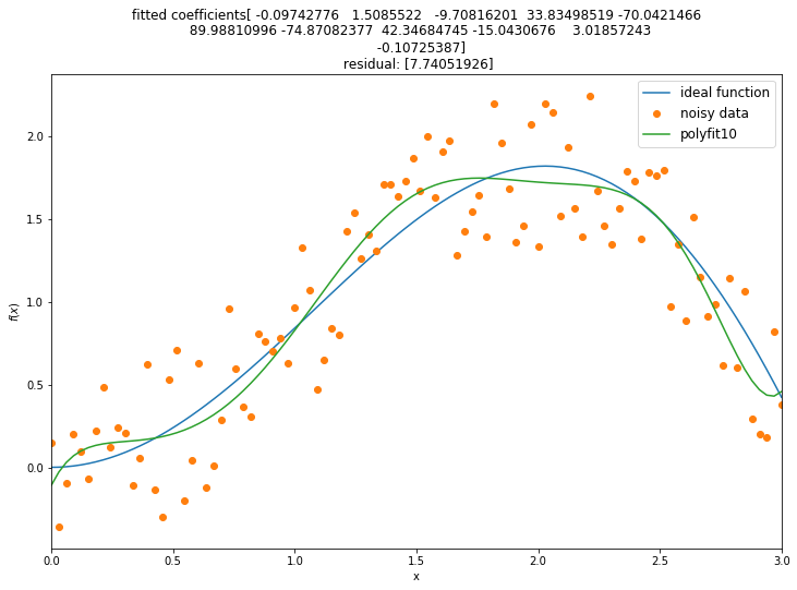
多項式フィッティング
Use with p = np.polyfit(x, y, pOrder) and np.ployval(p, x)
指定された x および y データを設定します
[ ]:
%matplotlib inline

import matplotlib.pyplot as plt
import numpy as np

plt.figure(figsize=[12, 8])
#define the function
f = lambda x: x * np.sin(x)

#define the paramters for the plot
a,b = 0,3
npoints = 100
order = 10

x = np.linspace(a,b,npoints)
y = f(x) + np.random.rand(npoints) - 0.5
Get a polyfit
polyval を使用して多項式を評価する
[ ]:
fit = np.polyfit(x, y, order, full=True)
y_p = np.polyval(fit[0], x)
[37]:
plt.plot(x,f(x), label='ideal function')
plt.plot(x,y, 'o', label='noisy data')
plt.plot(x,y_p, label='polyfit'+str(order))

plt.xlabel('x')
plt.ylabel('$f(x)$')
plt.xlim([a,b])
plt.legend(fontsize=12)
plt.title('fitted coefficients' + str(fit[0]) + '\n residual: ' + str(fit[1]))
plt.show()
#plt.text(2, 2, fit)
クイズ
異なる多項式関数でコードを実行してみて、どの多項式が最適かを判断してください。
[38]:
help(np.polyfit)
Help on function polyfit in module numpy.lib.polynomial:

polyfit(x, y, deg, rcond=None, full=False, w=None, cov=False)
    Least squares polynomial fit.

    Fit a polynomial ``p(x) = p[0] * x**deg + ... + p[deg]`` of degree `deg`
    to points `(x, y)`. Returns a vector of coefficients `p` that minimises
    the squared error.

    Parameters
    ----------
    x : array_like, shape (M,)
        x-coordinates of the M sample points ``(x[i], y[i])``.
    y : array_like, shape (M,) or (M, K)
        y-coordinates of the sample points. Several data sets of sample
        points sharing the same x-coordinates can be fitted at once by
        passing in a 2D-array that contains one dataset per column.
    deg : int
        Degree of the fitting polynomial
    rcond : float, optional
        Relative condition number of the fit. Singular values smaller than
        this relative to the largest singular value will be ignored. The
        default value is len(x)*eps, where eps is the relative precision of
        the float type, about 2e-16 in most cases.
    full : bool, optional
        Switch determining nature of return value. When it is False (the
        default) just the coefficients are returned, when True diagnostic
        information from the singular value decomposition is also returned.
    w : array_like, shape (M,), optional
        Weights to apply to the y-coordinates of the sample points. For
        gaussian uncertainties, use 1/sigma (not 1/sigma**2).
    cov : bool, optional
        Return the estimate and the covariance matrix of the estimate
        If full is True, then cov is not returned.

    Returns
    -------
    p : ndarray, shape (deg + 1,) or (deg + 1, K)
        Polynomial coefficients, highest power first.  If `y` was 2-D, the
        coefficients for `k`-th data set are in ``p[:,k]``.

    residuals, rank, singular_values, rcond
        Present only if `full` = True.  Residuals of the least-squares fit,
        the effective rank of the scaled Vandermonde coefficient matrix,
        its singular values, and the specified value of `rcond`. For more
        details, see `linalg.lstsq`.

    V : ndarray, shape (M,M) or (M,M,K)
        Present only if `full` = False and `cov`=True.  The covariance
        matrix of the polynomial coefficient estimates.  The diagonal of
        this matrix are the variance estimates for each coefficient.  If y
        is a 2-D array, then the covariance matrix for the `k`-th data set
        are in ``V[:,:,k]``


    Warns
    -----
    RankWarning
        The rank of the coefficient matrix in the least-squares fit is
        deficient. The warning is only raised if `full` = False.

        The warnings can be turned off by

        >>> import warnings
        >>> warnings.simplefilter('ignore', np.RankWarning)

    See Also
    --------
    polyval : Compute polynomial values.
    linalg.lstsq : Computes a least-squares fit.
    scipy.interpolate.UnivariateSpline : Computes spline fits.

    Notes
    -----
    The solution minimizes the squared error

    .. math ::
        E = \sum_{j=0}^k |p(x_j) - y_j|^2

    in the equations::

        x[0]**n * p[0] + ... + x[0] * p[n-1] + p[n] = y[0]
        x[1]**n * p[0] + ... + x[1] * p[n-1] + p[n] = y[1]
        ...
        x[k]**n * p[0] + ... + x[k] * p[n-1] + p[n] = y[k]

    The coefficient matrix of the coefficients `p` is a Vandermonde matrix.

    `polyfit` issues a `RankWarning` when the least-squares fit is badly
    conditioned. This implies that the best fit is not well-defined due
    to numerical error. The results may be improved by lowering the polynomial
    degree or by replacing `x` by `x` - `x`.mean(). The `rcond` parameter
    can also be set to a value smaller than its default, but the resulting
    fit may be spurious: including contributions from the small singular
    values can add numerical noise to the result.

    Note that fitting polynomial coefficients is inherently badly conditioned
    when the degree of the polynomial is large or the interval of sample points
    is badly centered. The quality of the fit should always be checked in these
    cases. When polynomial fits are not satisfactory, splines may be a good
    alternative.

    References
    ----------
    .. [1] Wikipedia, "Curve fitting",
           http://en.wikipedia.org/wiki/Curve_fitting
    .. [2] Wikipedia, "Polynomial interpolation",
           http://en.wikipedia.org/wiki/Polynomial_interpolation

    Examples
    --------
    >>> x = np.array([0.0, 1.0, 2.0, 3.0,  4.0,  5.0])
    >>> y = np.array([0.0, 0.8, 0.9, 0.1, -0.8, -1.0])
    >>> z = np.polyfit(x, y, 3)
    >>> z
    array([ 0.08703704, -0.81349206,  1.69312169, -0.03968254])

    It is convenient to use `poly1d` objects for dealing with polynomials:

    >>> p = np.poly1d(z)
    >>> p(0.5)
    0.6143849206349179
    >>> p(3.5)
    -0.34732142857143039
    >>> p(10)
    22.579365079365115

    High-order polynomials may oscillate wildly:

    >>> p30 = np.poly1d(np.polyfit(x, y, 30))
    /... RankWarning: Polyfit may be poorly conditioned...
    >>> p30(4)
    -0.80000000000000204
    >>> p30(5)
    -0.99999999999999445
    >>> p30(4.5)
    -0.10547061179440398

    Illustration:

    >>> import matplotlib.pyplot as plt
    >>> xp = np.linspace(-2, 6, 100)
    >>> _ = plt.plot(x, y, '.', xp, p(xp), '-', xp, p30(xp), '--')
    >>> plt.ylim(-2,2)
    (-2, 2)
    >>> plt.show()
より一般的なカーブ フィッティング
一般的な関数 f(x; a, b, c) を当てはめることができます。ここで、f は、与えられたデータのセットに対して最適化したいパラメーター a、b、c を持つ x の関数です。この関数は scipy.optimize から利用できます。以下は、関数 \(f(x)\) を次の式に適合させる例です
[43]:
from scipy.optimize import curve_fit
import matplotlib.pyplot as plt
import numpy as np

plt.figure(figsize=[10, 6])


#define the function
f = lambda x,a,b,c: a*np.exp(-b*x)+c

#define the paramters for the plot
x_min, x_max = 0, 10
npoints = 100
a,b,c = 2.5, 1.3, 0.4

x = np.linspace(x_min, x_max, npoints)
y = f(x,a,b,c) + np.random.rand(npoints) - 0.5

#do the curve fit
params, extras = curve_fit(f, x, y)

plt.plot(x,f(x,a,b,c), '--', label='ideal function')
plt.plot(x,y, 'o', label='noisy data')
plt.plot(x,f(x,params[0],params[1],params[2]), label='curve_fit')

plt.xlabel('x')
plt.ylabel('$f(x)$')
plt.xlim([x_min, x_max])
plt.legend(fontsize=12)
plt.show()
print('original coefficients: %6.3f, %6.3f, %6.3f' %(a,b,c))
print('fitted   coefficients: %6.3f, %6.3f, %6.3f' %(params[0], params[1], params[2]))
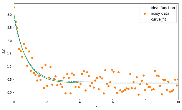
original coefficients:  2.500,  1.300,  0.400
fitted   coefficients:  2.686,  1.364,  0.359
発展
このセクションでは、最小二乗距離を使用して最も近い適合を表すことを学びました。それは常に最良の基準でしょうか?
他の基準もあります。scipy では、距離に関するさまざまな定義があります。
https://docs.scipy.org/doc/scipy-0.14.0/reference/generated/scipy.spatial.distance.pdist.html
https://www.cs.utah.edu/~jeffp/teaching/cs5955/L7-Distances.pdf
\(L_p\) distances
cosine
jaccard
ユークリッド距離 (\(L_2\)) は、最も一般的に使用される距離メトリックですが、決して唯一の定義ではありません。
場合によっては、\(L_1\) の距離の方が、さまざまな目的に適していることがあります。 たとえば、\(L_1\) は、高速信号/画像処理専用の新しいアルゴリズムで広く使用されています。
課題
次のことを行う独自のプログラムを作成します。 - ランダム ノイズを含むデータを生成する - データに適合するために別の多項式関数を選択する - どの多項式関数が最も適しているかを議論し、その理由を述べてください。
[ ]: