補間
補間は、データ解析で広く利用されています。積分や微分とは直接関係はありませんが、同様の数学的方法を使用します。
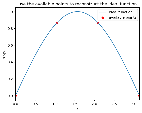
関数 \(f(x)\) の 2 点 \(x = a, b\) での値が与えられ、その間の別の点 \(x\) での関数の値を知りたいとします。 どうすれば良いと思いますか?
簡単な例として関数 \(f(x)\) が sin(x)である場合について考えてみましょう。
[1]:
import matplotlib.pyplot as plt
import numpy as np
from math import pi

f = lambda x: np.sin(x)
x_min, x_max = 0, pi
npt0 = 100
npt1 = 4

x0 = np.linspace(x_min, x_max, npt0)
x1 = np.linspace(x_min, x_max, npt1)

plt.plot(x0,f(x0),label='ideal function')
plt.scatter(x1,f(x1), color='r', label='available points')

plt.legend()
plt.xlabel('x')
plt.ylabel('sin(x)')
plt.xlim([0,pi])
#plt.title('いくつかの点から元の関数を再構築せよ')
plt.title('use the available points to reconstruct the ideal function')
plt.show()
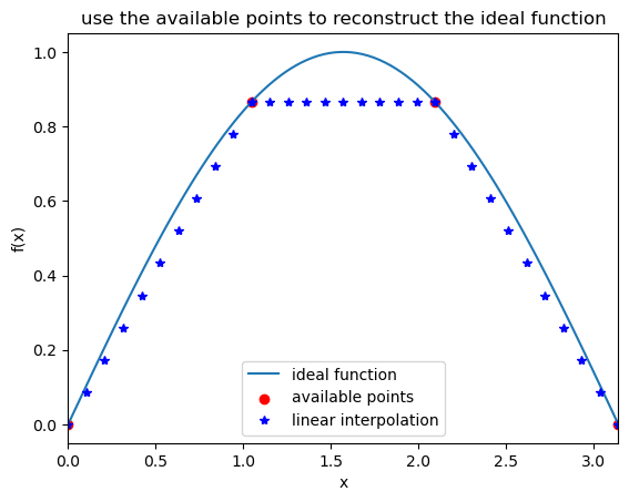
線形補間
最も単純なのは線形補間です。 関数は \(f(a)\) から \(f(b)\) への直線に従うと仮定します。現実には関数は 2 点間で曲線に従う可能性がありますが、この仮定では、いくつかの初等幾何学で \(f(x)\) を計算することができます。
直線近似の傾きは
これは、台形公式を用いた積分で行ったことと同じです。
[2]:
import matplotlib.pyplot as plt
import numpy as np
from math import pi

f = lambda x: np.sin(x)
x_min, x_max = 0, pi
npt0 = 100 #ideal function
npt1 = 4   #available points
npt2 = 10  #number of points you want to interpolate bewteen two known points

x0 = np.linspace(x_min, x_max, npt0) #ideal function
x1 = np.linspace(x_min, x_max, npt1) #available points


#---------To interpolate based on the available points

x2 = []
y2 = []

for i in range(npt1-1):
    slope = (f(x1[i+1])-f(x1[i]))/(x1[i+1]-x1[i])
    delta = (x1[i+1]-x1[i])/npt2
    for j in range(npt2+1):
        x2.append(x1[i]+delta*j)
        y2.append(f(x1[i]) + slope*delta*j)
#---------To interpolate based on the available points


#plot all points
plt.plot(x0,f(x0),label='ideal function')
plt.scatter(x1,f(x1), color='r', label='available points')
plt.plot(x2,y2, '*b', label='linear interpolation')

plt.legend()
plt.xlabel('x')
plt.ylabel('f(x)')
plt.xlim([0,pi])
plt.title('use the available points to reconstruct the ideal function')
plt.show()
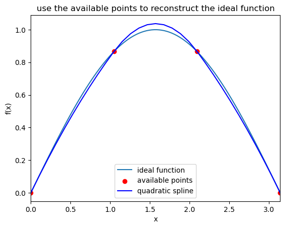
スプライン補間
理想的な関数が線形からかけ離れている場合には、線形補間は適切な近似ではありません。したがって、場合によっては重大なエラーが発生する可能性があります。
積分の時に行ったことと同様に、より精度の良い近似は多項式関数を使用することです。スプライン補間は、補間関数がスプラインと呼ばれる特殊なタイプの多項式である補間の形式です。
線形補間は、実際にはスプライン補間の最も単純なバージョンです。
二次スプライン補間を行う場合、関係はもう少し複雑になります。
簡単な例から始めましょう。\((-1,0), (0,1), (1,3)\)の3つの点があたえられていると仮定します。
求めたい二次スプラインは次のとおりです。
以下の条件を満たす必要があります。
さらに、曲線を連続にしたいので、 \(p_1(0)' = p_ 2(0)'\) は、
となります。
全部で 6 つの変数がありますが、式は 5 つしかないため、別の条件を定義する必要があります。
通常、両端の導関数についても制約を課すことができます。たとえば\(p_1(-1)'\)=0とすると、
したがって、方程式を解くことで二次スプライン関数のすべての係数を取得できます。
一連の点を補間すると、一般化された関係は次のようになります。
\(z\) シリーズは次の方法で取得できます
\(z_0\) は 1 番目の点の導関数です。
[3]:
import matplotlib.pyplot as plt
import numpy as np
from math import pi

f = lambda x: np.sin(x)
x_min, x_max = 0, pi
npt0 = 100 #ideal function
npt1 = 4   #available points
npt2 = 10  #number of points you want to interpolate bewteen two known points

x0 = np.linspace(x_min, x_max, npt0) #ideal function
x1 = np.linspace(x_min, x_max, npt1) #available points


#---------To interpolate based on the available points
x2 = []
y2 = []
z = np.empty(npt1)
z[0] = 1    # try to play with different values here

for i in range(npt1-1):
    slope = (f(x1[i+1])-f(x1[i]))/(x1[i+1]-x1[i])
    delta = (x1[i+1]-x1[i])/npt2
    z[i+1] = -z[i] + 2*slope


    for j in range(npt2+1):
        x2.append(x1[i]+delta*j)
        y2.append(f(x1[i]) + z[i]*delta*j + (z[i+1]-z[i])*delta*j*j/2/npt2)
        #print(x2[-1],y2[-1])
#---------To interpolate based on the available points


#plot all points
plt.plot(x0,f(x0),label='ideal function')
plt.scatter(x1,f(x1), color='r', label='available points')
plt.plot(x2,y2, 'b', label='quadratic spline')


plt.legend()
plt.xlabel('x')
plt.ylabel('f(x)')
plt.xlim([0,pi])
plt.title('use the available points to reconstruct the ideal function')
plt.show()
同様に、高次多項式も実行できます。 たとえば3 次スプラインは、多くの分野で使用されている一般的な方法です。 ロジックは、多項式関数と条件の拡張に他なりません。
ここで、$h_i = x_{i+1} - x_i $、および \(z\) シリーズは次の方法で取得できます。
Scipy の高度なライブラリ
実用上は、このようなコードをゼロから書くよりも、既にあるコードを理解する方が簡単です。 実際、3 次スプラインはすでにライブラリに実装されており、非常に便利なものになっています。
幸いなことに、科学的プログラミングのための基本的なライブラリが構築されています。 Python で最も重要なのは scipy です。
scipy を使用した後、ここで行ったようなれらの低レベルの作業は回避できることがすぐにわかります。しかし、少なくともこれらの機能の原理は知っておく必要があります。 何も知らずに関数を使うのは非常に危険です。
scipy での積分の例
[4]:
import numpy as np
from scipy import integrate

f = lambda x: 3*x**3 + 1
x_min, x_max = 0, 1
I, err = integrate.quad(f,x_min,x_max)
print(I, err)
1.75 1.942890293094024e-14
scipy での補間の例
[5]:
import matplotlib.pyplot as plt
import numpy as np
from math import pi
from scipy.interpolate import *
from random import random

f = lambda x: np.sin(x)+random()
x_min, x_max = 0, 2*pi
npt0 = 100 #ideal function
npt1 = 4   #available points
npt2 = 10  #number of points you want to interpolate bewteen two known points

x0 = np.linspace(x_min, x_max, npt0) #ideal function
x1 = np.linspace(x_min, x_max, npt1) #available points

f_spline1 = interpolate.interp1d(x1, f(x1), kind='linear')
f_spline2 = interpolate.interp1d(x1, f(x1), kind='quadratic')
f_spline3 = interpolate.interp1d(x1, f(x1), kind='cubic')


#plot all points
plt.plot(x0,f(x0),label='ideal function')
plt.plot(x0,f_spline1(x0), '--',  label='linear')
plt.plot(x0,f_spline2(x0), '-', label='quadratic')
plt.plot(x0,f_spline3(x0), '-.', label='cubic')
plt.scatter(x1,f(x1), c='r', s=180, marker='*', label='available points')


plt.legend()
plt.xlabel('x')
plt.ylabel('f(x)')
plt.xlim([x_min, x_max])
plt.title('interpolation with built-in function in scipy')
plt.show()
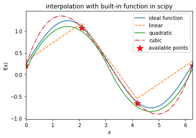
補完における次数の選び方
曲線が連続的であるためには、各セグメントが出会ったときに等しい値を与えることを確認する必要があります
\(f_i(x_i) = f_{i+1}(x_i)\)
これが線形スプラインの機能です。
曲線を滑らかにするために、1次導関数が等しくなるように求めます
\((f_i(x_i))' = (f_{i+1}(x_i))'\)
これは二次スプライン補間で使用されています。
セグメントが接するときに同じ曲率を持つようにするには、以下を課します。
\((f_i(x_i))'' = (f_{i+1}(x_i))''\)
この条件を満たすには、3 次スプラインを使用する必要があります。 これが、人々が補間を行うときに 3 次スプラインが最も一般的な選択肢である理由です。
高次の方程式はさらに滑らかな曲線を与えますが、コストが高くなり、変化がより微妙になります。精度と複雑さの間にはトレードオフがあります。
[6]:
import matplotlib.pyplot as plt

x = np.linspace(0,10, 100)
plt.plot(x, x, label='y=x')
plt.show()
[7]:
x = np.linspace(-10, 10, 100)
plt.plot(x, x**3 - 2*x**2- 10*x + 20, label='2nd')
plt.show()
[ ]: