誤差の評価 (Uncertainty quantification)
MCMCシミュレーションでは、ベイズ推定により事後分布を最大化するパラメータセットを求めるが、この最適なパラメータセットは熱力学パラメータの期待値に対応する。
その過程でモンテカルロシミュレーションを導入することにより、最適ではないがある程度もっともらしいパラメータセットも同時に獲得しており、これにより熱力学パラメータの標準偏差を評価することができる。これがUncertainty quantification(誤差の評価)である。
MCMCデータ
事前に用意されたtrace (Cr-Ni-trace.npy)とlnprob (Cr-Ni-lnprob.npy) を使用する。chains, itarations, parametersはそれぞれ40, 1000, 10である。不確実性の定量化を行うのに十分なサンプルを持つ完全に収束した MCMC シミュレーションには、数百から数千の計算が必要になります。40個のchainsをサンプリングし、1000回のitarationsを行い、パラメータ空間で合計40,000個のサンプルを取得した場合、2015年製MacBook Pro(2.2GHz Intel
i7)の6コアで実行するのに3.5時間かかっています。
[2]:
import time
import matplotlib.pyplot as plt
import numpy as np
#import xarray as xr
import corner
from pycalphad import Database, equilibrium, variables as v
from pycalphad.plot.utils import phase_legend
from espei.datasets import load_datasets, recursive_glob
from espei.utils import database_symbols_to_fit, optimal_parameters
#from uq_helpers import highest_density_parameters, format_parameter_symbols

#pycalphad
dbf = Database('mcmc-start.tdb')
comps = ['CR', 'NI']
datasets = load_datasets(recursive_glob('input-data', '*.json'))

#espei
trace = np.load('Cr-Ni-trace.npy')
lnprob = np.load('Cr-Ni-lnprob.npy')
symbols_to_fit = database_symbols_to_fit(dbf)

print(trace.shape)
print(lnprob.shape)
(40, 1000, 10)
(40, 1000)
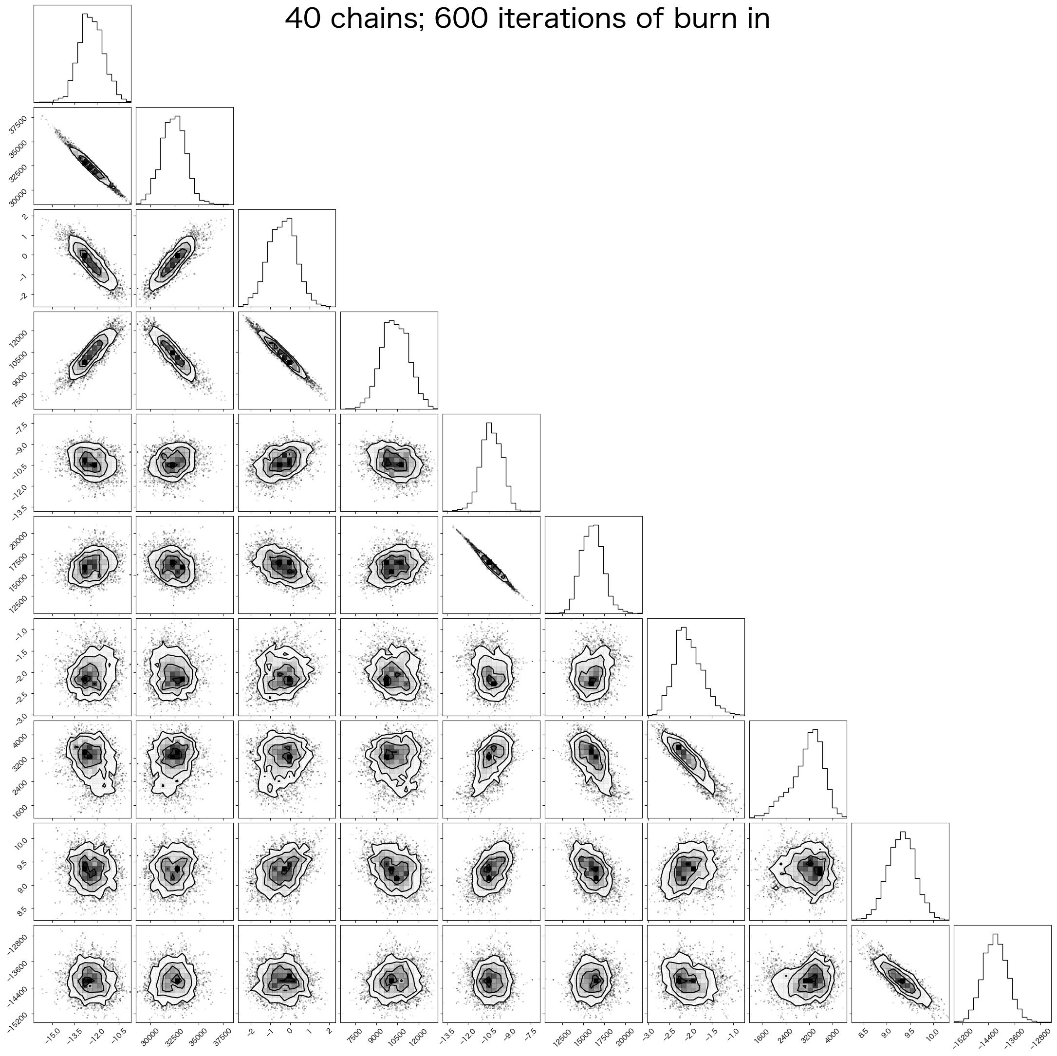
Corner plot
このPythonモジュールは、matplotlibを用いて散布図行列で多次元サンプルを可視化します。これらの可視化では、サンプルの1次元および2次元の各投影がプロットされ、共分散が明らかになります。cornerは元々、マルコフ連鎖モンテカルロシミュレーションの結果を表示するために考案されました。デフォルトはこの用途を念頭に置いて選択されていますが、質的に異なる様々なサンプルの表示にも使用できます。
cornerの開発はGitHub上で行われているため、問題があればGitHubで報告できます。cornerは天文学の文献で広く使用されており、corner.py、または以前の名前であるtriangle.pyとして引用されることもあります。
[3]:
burnin = 600  # first non-burn-in index (discard previous)

# flatten the along the first dimension containing all the chains in parallel
#fig = corner.corner(trace[:,burnin:,:].reshape(-1, trace[:,burnin:,:].shape[-1]), labels=format_parameter_symbols(dbf), label_kwargs={'fontsize': 20})
fig = corner.corner(trace[:,burnin:,:].reshape(-1, trace[:,burnin:,:].shape[-1]), label_kwargs={'fontsize': 20})
fig.suptitle(f"{trace.shape[0]} chains; {burnin} iterations of burn in", fontsize=40)
[3]:
Text(0.5, 0.98, '40 chains; 600 iterations of burn in')
結局のところ、探索すべき機能は数多くあり、ここではいくつかの基本的な機能についてのみ説明しました。結果はすべて配列として保存されるため、適切な手法を用いて自由に分析できます。
誤差の伝搬 (Uncertainty propagation)
最適なパラメータセットは熱力学量の期待値に評価するために使用されるが、一方で、最適ではないパラメータセットも重要な活用方法がある。これらを使用して熱力学量を計算すると、熱力学量にもばらつきが生じることとなり、これは熱力学パラメータの誤差が、熱力学量へ伝搬する振舞いを表現する。
従来の最適なパラメータセットのみで計算した状態図は、このような誤差が正しく表現されていない点において不十分であると考える。ここではこのようなUncertainty propagationの評価方法について説明する。
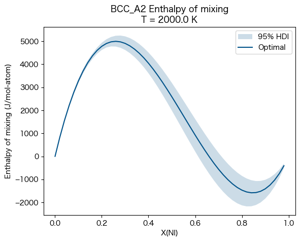
混合エンタルピー (enthalpy of mixing)
ここではBCC_A2相の enthalpy of mixing(混合エンタルピー)に伝搬する誤差の評価を行う。
これにはuq_helpers.pyに含まれる95%信頼区間を求めるhighest_density_parametersを使用する。
highest_density_parameters
credible_interval(信頼区間)に従って最も高い密度を持つtraceを返します。traceは2次元の配列であり、形式は(samples, parameters)です。ここでは以下のように指定しています。
flat_params = highest_density_parameters(trace, lnprob, burn_in=600, thin=200)
trace
MCMCシミュレーションで得られたtrace: 3D array of shape (chains, iterations, parameters)
lnprob
MCMCシミュレーションで得られたlnprob: 2D array of shape (chains, iterations)
credible_interval
考慮するhighest density pointsを 0 ~ 1 で指定する。0.95 の場合、95% HDI (Highest Density Interval) に対応。
burn_in
burn inとして考慮する反復回数。上の例では600回目までは使用しない。
thin
n番目ごとにサンプルを取得する。上の例では200番目毎にサンプルを取得する。
[14]:
import xarray as xr
from uq_helpers import highest_density_parameters, format_parameter_symbols

phases = ['BCC_A2']
conds = {v.P: 101325, v.N: 1, v.T: 2000.0, v.X('NI'): (0, 1, 0.02)}
#for calculate
#conds = {v.P: 101325, v.T: 2000.0, v.X('NI'): (0, 1, 0.02)}
prop = 'HM_MIX'

#
flat_params = highest_density_parameters(trace, lnprob, burn_in=600, thin=200)
95% HDIを満足するパラメータセットの数を確認します。
[15]:
flat_params.shape
[15]:
(76, 10)
このflat_paramsに対してpycalphadのequilibriumを使用してHM_MIXを求めます。
Note:平衡計算ではないので本来はcalculateを使用するべきと思うが、equilibriumが使用されている。calculateは以下のようにequilibriumとは引数が異なっている、単純にcalculateに置き換えるだけでは計算ができない。統一的にequilibriumを使用するのが良い。
calculate(dbf, comps, phase, P=101325, T=(500, 1100, 100))
equilibrium(dbf, comps , phases, {v.X('ZN'):(0,1,0.05), v.T: (500, 1000, 100), v.P:101325}, output='HM')
[26]:
from pycalphad import calculate

# Loop over all the parameter sets in flat_params and perform the foward (propagation) calculation
t1 = time.time()
eq_results = []
for param_idx in range(flat_params.shape[0]):
    parameters = dict(zip(symbols_to_fit, flat_params[param_idx, :]))
    eq_res = equilibrium(dbf, comps, phases, conds, output=prop, parameters=parameters)
    #for calculate
    #eq_res = calculate(dbf, comps, phases, conds, output=prop, parameters=parameters)
    eq_results.append(eq_res)

print(f'Time to compute equilibrium uncertainty for {prop} with conditions {conds}: {time.time() - t1:0.2f} seconds')

# Concatenate all the parameter samples on a new dimension
eq_up_result = xr.concat(eq_results, 'samples')

# Compute the "optimal" property
params = dict(zip(database_symbols_to_fit(dbf), optimal_parameters(trace, lnprob)))
dbf.symbols.update(params)
eq_opt_result = equilibrium(dbf, comps, phases, conds, output=prop, parameters=params)
Time to compute equilibrium uncertainty for HM_MIX with conditions {P: 101325, T: 2000.0, X_NI: (0, 1, 0.02), N: 1}: 1.05 seconds
[27]:
print(eq_up_result)
<xarray.Dataset>
Dimensions:    (samples: 76, N: 1, P: 1, T: 1, X_NI: 50, vertex: 3,
                component: 2, internal_dof: 2)
Coordinates:
  * N          (N) float64 1.0
  * P          (P) float64 1.013e+05
  * T          (T) float64 2e+03
  * X_NI       (X_NI) float64 1e-10 0.02 0.04 0.06 0.08 ... 0.92 0.94 0.96 0.98
  * vertex     (vertex) int64 0 1 2
  * component  (component) <U2 'CR' 'NI'
Dimensions without coordinates: samples, internal_dof
Data variables:
    NP         (samples, N, P, T, X_NI, vertex) float64 1.0 nan nan ... nan nan
    GM         (samples, N, P, T, X_NI) float64 -1.071e+05 ... -1.244e+05
    MU         (samples, N, P, T, X_NI, component) float64 -1.071e+05 ... -1....
    X          (samples, N, P, T, X_NI, vertex, component) float64 1.0 ... nan
    Y          (samples, N, P, T, X_NI, vertex, internal_dof) float64 1.0 ......
    Phase      (samples, N, P, T, X_NI, vertex) <U6 'BCC_A2' '' '' ... '' ''
    HM_MIX     (samples, N, P, T, X_NI) float64 4.289e-06 816.1 ... -454.7
Attributes:
    engine:   pycalphad 0.10.2
    created:  2025-05-29T06:12:50.759804
[28]:
_hndls, colors = phase_legend(phases)
eq_prop = eq_up_result[prop].squeeze()
fig = plt.figure()
ax = fig.add_subplot()

# Single phase assumption (no miscibility gap)
ax.fill_between(eq_up_result.X_NI, eq_prop.min(dim='samples'), eq_prop.max(dim='samples'), alpha=0.2, color=colors[phases[0]], edgecolor=None, label='95% HDI')
ax.plot(eq_opt_result.X_NI, eq_opt_result[prop].squeeze(), color=colors[phases[0]], label='Optimal')
#for calculate
#ax.fill_between(eq_up_result.X, eq_prop.min(dim='samples'), eq_prop.max(dim='samples'), alpha=0.2, color=colors[phases[0]], edgecolor=None, label='95% HDI')
#ax.plot(eq_opt_result.X, eq_opt_result[prop].squeeze(), color=colors[phases[0]], label='Optimal')
ax.set_title(f'{phases[0]} Enthalpy of mixing\nT = {conds[v.T]} K')
ax.set_ylabel('Enthalpy of mixing (J/mol-atom)')
ax.set_xlabel('X(NI)')
ax.legend(loc=0)
[28]:
<matplotlib.legend.Legend at 0x30a706250>
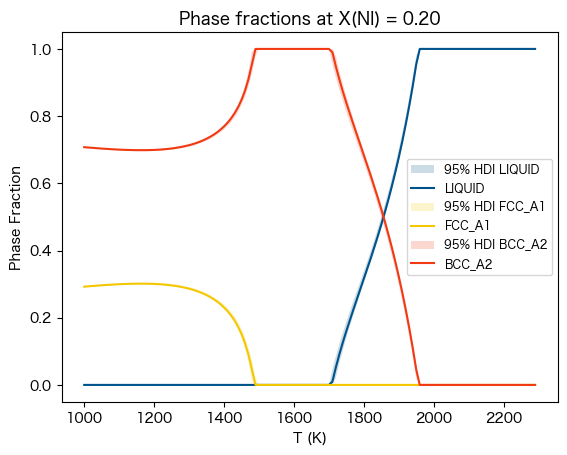
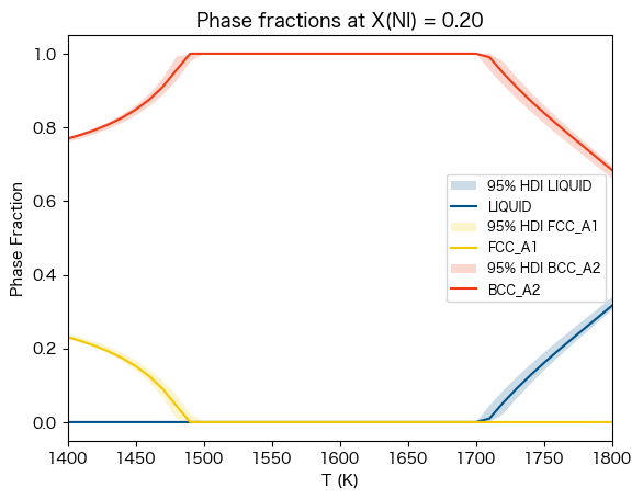
相分率 (Phase Fraction vs. Temperature)
ここではLIQUID, FCC_A1, BCC_A2相の enthalpy of mixing(混合エンタルピー)に伝搬する誤差の評価を行う。
これにはuq_helpers.pyに含まれる95%信頼区間を求めるhighest_density_parametersを使用する。
[29]:
phases = ['LIQUID', 'FCC_A1', 'BCC_A2']
conds = {v.P: 101325, v.N: 1, v.T: (1000, 2300, 10), v.X('NI'): 0.20}
flat_params = highest_density_parameters(trace, lnprob, burn_in=600, thin=500)
[30]:
flat_params.shape
[30]:
(31, 10)
[31]:
# Loop over all the parameter sets in flat_params and perform the foward (propagation) calculation
t1 = time.time()
eq_results = []
for param_idx in range(flat_params.shape[0]):
    parameters = dict(zip(symbols_to_fit, flat_params[param_idx, :]))
    eq_res = equilibrium(dbf, comps, phases, conds, parameters=parameters)
    eq_results.append(eq_res)
print(f'Time to compute equilibrium uncertainty for NP with conditions {conds}: {time.time() - t1:0.2f} seconds')

# Concatenate all the parameter samples on a new dimension
eq_up_result = xr.concat(eq_results, 'samples')

# Compute the "optimal" property
params = dict(zip(database_symbols_to_fit(dbf), optimal_parameters(trace, lnprob)))
dbf.symbols.update(params)
eq_opt_result = equilibrium(dbf, comps, phases, conds, parameters=params)
Time to compute equilibrium uncertainty for NP with conditions {P: 101325, N: 1, T: (1000, 2300, 10), X_NI: 0.2}: 1.26 seconds
[32]:
print(eq_up_result)
<xarray.Dataset>
Dimensions:    (samples: 31, N: 1, P: 1, T: 130, X_NI: 1, vertex: 3,
                component: 2, internal_dof: 2)
Coordinates:
  * N          (N) float64 1.0
  * P          (P) float64 1.013e+05
  * T          (T) float64 1e+03 1.01e+03 1.02e+03 ... 2.28e+03 2.29e+03
  * X_NI       (X_NI) float64 0.2
  * vertex     (vertex) int64 0 1 2
  * component  (component) <U2 'CR' 'NI'
Dimensions without coordinates: samples, internal_dof
Data variables:
    NP         (samples, N, P, T, X_NI, vertex) float64 0.7053 0.2947 ... nan
    GM         (samples, N, P, T, X_NI) float64 -3.93e+04 ... -1.469e+05
    MU         (samples, N, P, T, X_NI, component) float64 -3.677e+04 ... -1....
    X          (samples, N, P, T, X_NI, vertex, component) float64 0.9903 ......
    Y          (samples, N, P, T, X_NI, vertex, internal_dof) float64 0.9903 ...
    Phase      (samples, N, P, T, X_NI, vertex) <U6 'BCC_A2' 'FCC_A1' ... '' ''
Attributes:
    engine:   pycalphad 0.10.2
    created:  2025-05-29T06:16:48.556047
[8]:
_hndls, colors = phase_legend(phases)
prop = 'NP'
fig = plt.figure()
ax = fig.add_subplot()
for phase_name in phases:
    msk = eq_up_result.Phase == phase_name
    eq_prop = eq_up_result[prop].where(msk).sum(dim='vertex').squeeze()  # WARNING: sum here implies no miscibility gaps
    ax.fill_between(eq_up_result.T, eq_prop.min(dim='samples'), eq_prop.max(dim='samples'), alpha=0.2, color=colors[phase_name], edgecolor=None, label=f'95% HDI {phase_name}')
    ax.plot(eq_opt_result.T, eq_opt_result[prop].where(eq_opt_result.Phase == phase_name).sum(dim='vertex').squeeze(), label=phase_name, color=colors[phase_name])
ax.set_title(f'Phase fractions at X(NI) = {conds[v.X("NI")]:0.2f}')
ax.set_ylabel('Phase Fraction')
ax.set_xlabel('T (K)')
ax.legend(loc=0, fontsize='small')
[8]:
<matplotlib.legend.Legend at 0x1694fd1f0>
[9]:
_hndls, colors = phase_legend(phases)
prop = 'NP'

fig = plt.figure()
ax = fig.add_subplot()
for phase_name in phases:
    msk = eq_up_result.Phase == phase_name
    eq_prop = eq_up_result[prop].where(msk).sum(dim='vertex').squeeze()  # WARNING: sum here implies no miscibility gaps
    ax.fill_between(eq_up_result.T, eq_prop.min(dim='samples'), eq_prop.max(dim='samples'), alpha=0.2, color=colors[phase_name], edgecolor=None, label=f'95% HDI {phase_name}')
    ax.plot(eq_opt_result.T, eq_opt_result[prop].where(eq_opt_result.Phase == phase_name).sum(dim='vertex').squeeze(), label=phase_name, color=colors[phase_name])
ax.set_title(f'Phase fractions at X(NI) = {conds[v.X("NI")]:0.2f}')
ax.set_ylabel('Phase Fraction')
ax.set_xlabel('T (K)')
ax.legend(loc=0, fontsize='small')
ax.set_xlim(1400, 1800)
[9]:
(1400.0, 1800.0)
[ ]:
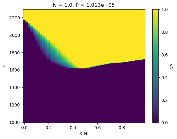
相境界 (Phase boundary)
ここではLIQUID, FCC_A1, BCC_A2相の Phase boundary(相境界)に伝搬する誤差の評価を行う。
これにはuq_helpers.pyに含まれる95%信頼区間を求めるhighest_density_parametersを使用する。
[2]:
import time
import matplotlib.pyplot as plt
import numpy as np
import xarray as xr
import corner
from pycalphad import Database, equilibrium, variables as v
from pycalphad.plot.utils import phase_legend
from espei.datasets import load_datasets, recursive_glob
from espei.utils import database_symbols_to_fit, optimal_parameters
from uq_helpers import highest_density_parameters, format_parameter_symbols

#pycalphad
dbf = Database('mcmc-start.tdb')
comps = ['CR', 'NI']
datasets = load_datasets(recursive_glob('input-data', '*.json'))

#espei
trace = np.load('Cr-Ni-trace.npy')
lnprob = np.load('Cr-Ni-lnprob.npy')
symbols_to_fit = database_symbols_to_fit(dbf)

phases = ['LIQUID', 'FCC_A1', 'BCC_A2']
conds = {v.P: 101325, v.N: 1, v.T: (1000, 2300, 10), v.X('NI'): (0, 1, 0.02)}
flat_params = highest_density_parameters(trace, lnprob, burn_in=600, thin=500)
[3]:
samples, params=flat_params.shape
print("samples:",samples)
print("params:",params)
samples: 31
params: 10
[4]:
# Loop over all the parameter sets in flat_params and perform the foward (propagation) calculation
t1 = time.time()
eq_results = []
for param_idx in range(flat_params.shape[0]):
    parameters = dict(zip(symbols_to_fit, flat_params[param_idx, :]))
    eq_res = equilibrium(dbf, comps, phases, conds, parameters=parameters)
    eq_results.append(eq_res)
print(f'Time to compute equilibrium uncertainty for NP with conditions {conds}: {time.time() - t1:0.2f} seconds')

# Concatenate all the parameter samples on a new dimension
eq_up_result = xr.concat(eq_results, 'samples')

# Compute the "optimal" property
params = dict(zip(database_symbols_to_fit(dbf), optimal_parameters(trace, lnprob)))
dbf.symbols.update(params)
eq_opt_result = equilibrium(dbf, comps, phases, conds, parameters=params)
Time to compute equilibrium uncertainty for NP with conditions {P: 101325, N: 1, T: (1000, 2300, 10), X_NI: (0, 1, 0.02)}: 50.06 seconds
[5]:
print(eq_up_result)
<xarray.Dataset>
Dimensions:    (samples: 31, N: 1, P: 1, T: 130, X_NI: 50, vertex: 3,
                component: 2, internal_dof: 2)
Coordinates:
  * N          (N) float64 1.0
  * P          (P) float64 1.013e+05
  * T          (T) float64 1e+03 1.01e+03 1.02e+03 ... 2.28e+03 2.29e+03
  * X_NI       (X_NI) float64 1e-10 0.02 0.04 0.06 0.08 ... 0.92 0.94 0.96 0.98
  * vertex     (vertex) int64 0 1 2
  * component  (component) <U2 'CR' 'NI'
Dimensions without coordinates: samples, internal_dof
Data variables:
    NP         (samples, N, P, T, X_NI, vertex) float64 1.0 nan nan ... nan nan
    GM         (samples, N, P, T, X_NI) float64 -3.669e+04 ... -1.593e+05
    MU         (samples, N, P, T, X_NI, component) float64 -3.669e+04 ... -1....
    X          (samples, N, P, T, X_NI, vertex, component) float64 1.0 ... nan
    Y          (samples, N, P, T, X_NI, vertex, internal_dof) float64 1.0 ......
    Phase      (samples, N, P, T, X_NI, vertex) <U6 'BCC_A2' '' '' ... '' ''
Attributes:
    engine:   pycalphad 0.10.2
    created:  2025-06-03T03:10:40.100484
[6]:
eq_up_result['NP']
[6]:
<xarray.DataArray 'NP' (samples: 31, N: 1, P: 1, T: 130, X_NI: 50, vertex: 3)>
array([[[[[[1.        ,        nan,        nan],
           [0.98398651, 0.01601349,        nan],
           [0.95301693, 0.04698307,        nan],
           ...,
           [1.        ,        nan,        nan],
           [1.        ,        nan,        nan],
           [1.        ,        nan,        nan]],

          [[1.        ,        nan,        nan],
           [0.98492433, 0.01507567,        nan],
           [0.95375753, 0.04624247,        nan],
           ...,
           [1.        ,        nan,        nan],
           [1.        ,        nan,        nan],
           [1.        ,        nan,        nan]],

          [[1.        ,        nan,        nan],
           [0.98592889, 0.01407111,        nan],
           [0.95456008, 0.04543992,        nan],
           ...,
...
           ...,
           [1.        ,        nan,        nan],
           [1.        ,        nan,        nan],
           [1.        ,        nan,        nan]],

          [[1.        ,        nan,        nan],
           [1.        ,        nan,        nan],
           [1.        ,        nan,        nan],
           ...,
           [1.        ,        nan,        nan],
           [1.        ,        nan,        nan],
           [1.        ,        nan,        nan]]]]]])
Coordinates:
  * N        (N) float64 1.0
  * P        (P) float64 1.013e+05
  * T        (T) float64 1e+03 1.01e+03 1.02e+03 ... 2.27e+03 2.28e+03 2.29e+03
  * X_NI     (X_NI) float64 1e-10 0.02 0.04 0.06 0.08 ... 0.92 0.94 0.96 0.98
  * vertex   (vertex) int64 0 1 2
Dimensions without coordinates: samples[15]:
eq_up_result['NP'].sum(dim='vertex').sum('samples').shape
[15]:
(1, 1, 130, 50)
[17]:
print(eq_up_result['NP'].sum(dim='vertex').sum('samples'))
<xarray.DataArray 'NP' (N: 1, P: 1, T: 130, X_NI: 50)>
array([[[[31., 31., 31., ..., 31., 31., 31.],
         [31., 31., 31., ..., 31., 31., 31.],
         [31., 31., 31., ..., 31., 31., 31.],
         ...,
         [31., 31., 31., ..., 31., 31., 31.],
         [31., 31., 31., ..., 31., 31., 31.],
         [31., 31., 31., ..., 31., 31., 31.]]]])
Coordinates:
  * N        (N) float64 1.0
  * P        (P) float64 1.013e+05
  * T        (T) float64 1e+03 1.01e+03 1.02e+03 ... 2.27e+03 2.28e+03 2.29e+03
  * X_NI     (X_NI) float64 1e-10 0.02 0.04 0.06 0.08 ... 0.92 0.94 0.96 0.98
[7]:
eq_up_result['NP'].where(eq_up_result['NP']==1).sum(dim='vertex').sum('samples')
[7]:
<xarray.DataArray 'NP' (N: 1, P: 1, T: 130, X_NI: 50)>
array([[[[18.,  0.,  0., ..., 12., 19., 16.],
         [14.,  0.,  0., ..., 18., 17., 16.],
         [19.,  0.,  0., ..., 13., 13., 15.],
         ...,
         [ 9., 14., 17., ..., 18., 16., 13.],
         [15., 15., 15., ..., 20., 13., 18.],
         [19., 17., 17., ..., 14., 14., 16.]]]])
Coordinates:
  * N        (N) float64 1.0
  * P        (P) float64 1.013e+05
  * T        (T) float64 1e+03 1.01e+03 1.02e+03 ... 2.27e+03 2.28e+03 2.29e+03
* X_NI (X_NI) float64 1e-10 0.02 0.04 0.06 0.08 ... 0.92 0.94 0.96 0.98[9]:
#(eq_up_result['NP'].where(eq_up_result['NP']>0.99).where(eq_up_result['Phase']=='LIQUID').sum('vertex').sum('samples')/samples).plot()
(eq_up_result['NP'].where(eq_up_result['Phase']=='LIQUID').sum('vertex').sum('samples')/samples).plot()
[9]:
<matplotlib.collections.QuadMesh at 0x373e9a8e0>
[10]:
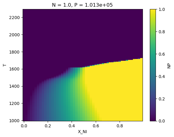
#(eq_up_result['NP'].where(eq_up_result['NP']>0.99).where(eq_up_result['Phase']=='FCC_A1').sum('vertex').sum('samples')/samples).plot()
(eq_up_result['NP'].where(eq_up_result['Phase']=='FCC_A1').sum('vertex').sum('samples')/samples).plot()
[10]:
<matplotlib.collections.QuadMesh at 0x373f54be0>
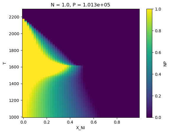
[11]:
#(eq_up_result['NP'].where(eq_up_result['NP']>0.99).where(eq_up_result['Phase']=='BCC_A2').sum('vertex').sum('samples')/samples).plot()
(eq_up_result['NP'].where(eq_up_result['Phase']=='BCC_A2').sum('vertex').sum('samples')/samples).plot()
[11]:
<matplotlib.collections.QuadMesh at 0x374009be0>
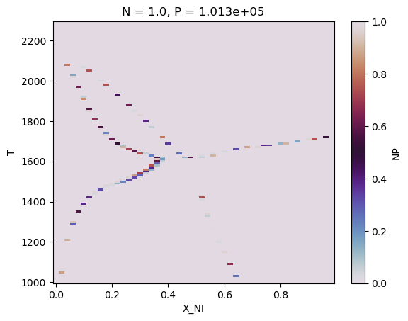
[19]:
(eq_up_result['NP'].where(eq_up_result['NP']>0.99).sum('vertex').sum('samples')/samples).plot(cmap='twilight')
#(eq_up_result['NP'].sum('vertex').sum('samples')/samples).plot()
[19]:
<matplotlib.collections.QuadMesh at 0x3745c4190>